In order to understand relationships between texts we often turn to the hclust function to create a dendrogram. This post will explain what is happening with that algorithm and how to explore its functionality with the built-in data on U.S. Cities. This tutorial can be used in conjunction with DCS 1200 “Data Driven Societies” and DCS/ENVS 2331 “The Nature of Data: Resource Management in the Digital Age”. Look for a Jupyter notebook with the R code so that you can follow along – coming soon!
One of the most frequent kinds of data used in text analysis is a distance matrix, which can be an odd configuration of information for users who aren’t used to working with a printed road atlas that would indicate the miles between different cities on a map. We’ll start with what is happening in two dimensions and then build on that to understand what is happening in the multiple dimensions of textual features that we measure.
The sample data for our function hclust considers 10 U.S. cities and we want to find pairs or clusters of cities that are similarly distant to the other cities in our data set:
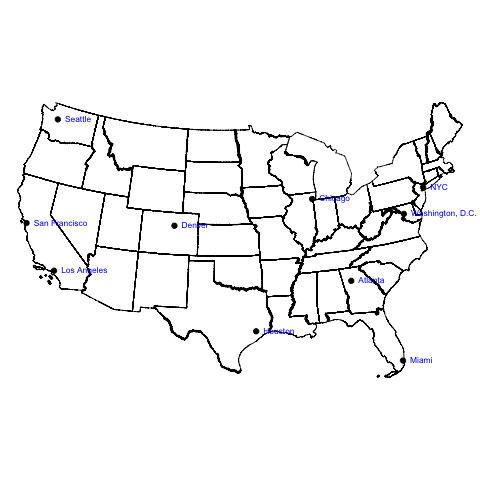
Typically we would think about regions in order to categorize the cities: NYC, D.C. and maybe Chicago in the Northeast; Atlanta, Miami, and maybe Houston in the Southeast, etc. Hclust considers the linear distance between the points, seen here in the two dimensions of longitude (x-axis) and latitude (y-axis).
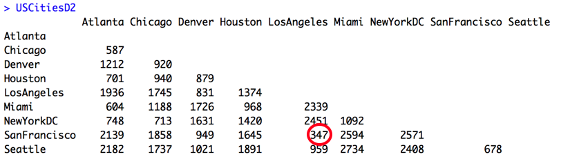
We would expect cities that are close together on the map to be similarly distant to the rest of the map. For example, San Francisco and Los Angeles on the West Coast are going to have relatively similar distances to cities on the East Coast. The distance between the cities can be represented as a matrix and we can see that San Francisco to New York is 2571 miles, LA to New York (or New York to LA in the data below) is 2451 miles, very similar:
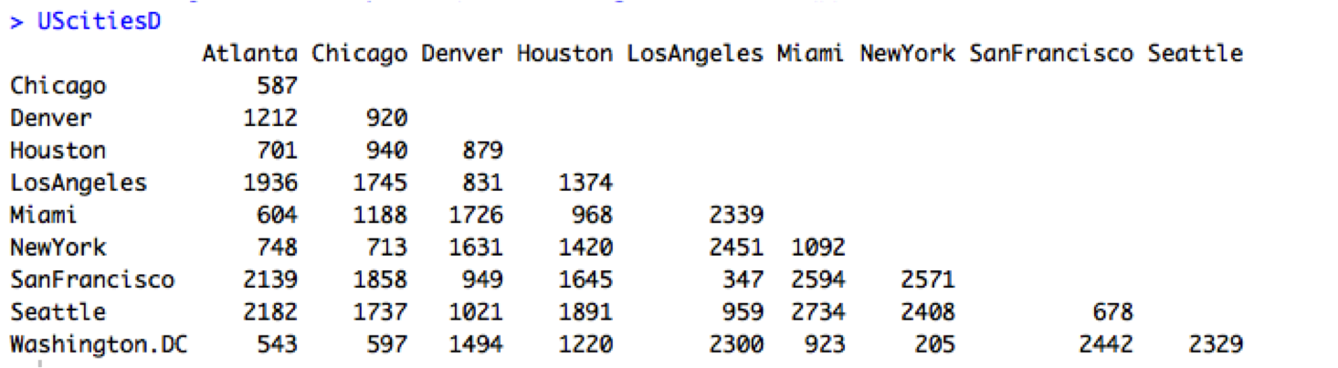
What happens when we compare each city’s distances to every other city’s distances? To find pairs like the obvious San Fran-L.A. cluster, we need to find cities that have a low difference in distances to each other, which by extension means finding similarly distant cities. We can think about our distance table as a dissimilarity matrix that shows the differences between the x and y values in our data (here the Euclidean or linear distance between two points). The lowest value will help to identify the lowest dissimilarity, which establishes the first pair in the cluster.
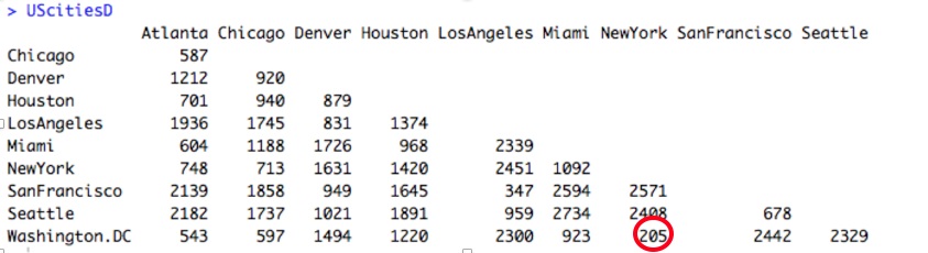
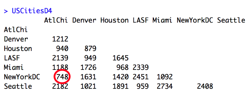
You will see that when we visualize the city clusters below in the final image, the New York – Washington, D.C. pair is together with a cluster height of 205 (indicated by a dashed red line). We can reduce our distance matrix to fewer columns by combining NY and DC. Using the complete or maximum linkage method we will keep the highest distance value to every other city in the data:

Our new distance matrix with the NewYork-DC cluster will look like the one below. Then we must keep searching for similarly distant pairs by finding the next two cities with the lowest distance between one another:
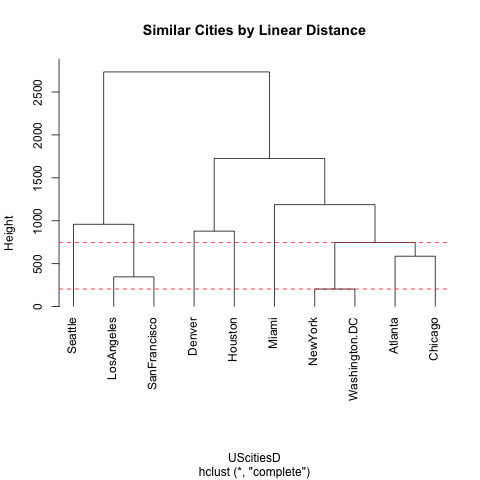
Los Angeles and San Francisco will appear as a cluster connected by a horizontal bar at height 347 to indicate their dissimilarity. Once we repeat these steps a few times, our most similar (or least dissimilar) pair will be a pair of clusters:
This means that the Atlanta-Chicago and New York-Washington, D.C. clusters will be joined by a horizontal bar at the height of 748 to indicate their dissimilarity (distance). When we put everything together to view these clusters in a dendrogram, we can see these similarly distant pairs:
We have rearranged our longitude-latitude (our x-y) data in such a way as to see new relationships. What happens when we apply this method to textual features? Instead of longitude on the x-axis, we might plot the relative frequency of the most frequent word (MFW) in our texts, and on the y-axis the relative frequency of the second most frequent word, and thanks to computation, we can continue this for 100 or 200 features (MFWs) into 100 or 200 dimensions. The algorithm then identifies the documents that are similarly distant, based on the same math that we have just outlined here. (You have seen this demonstrated in class and lab, but for another example, in a non-English language, see Prof. Hall’s work on computational parallax.) The biggest challenge is that we know a lot about the geographic space that separates cities and influences the features of those cities (although there is still much to learn), but we are only just starting to explore this computational aspect of the multi-dimensional space of texts.